WP-1500.1 and WP-1500.2
The main objective of the two tasks was to enable the EMM infrastructure to carry out impact studies and to perform end-to-end simulations of existing and future space missions remotely sensing the Earth’s atmosphere. The objective was pursued with two activities: on one hand, adequate high-performance computing resources were procured. On the other hand, some relevant open software modules were installed, characterized and advanced to build a set of tools suitable to carry out the mentioned studies and simulations.
Hardware
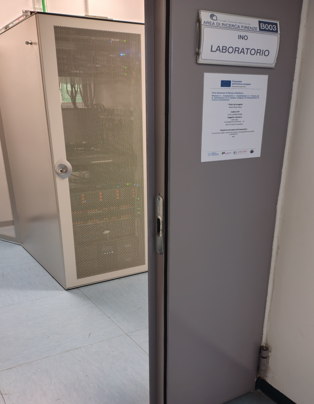
The hardware now available at CNR Research Area in Sesto Fiorentino (FI), INO computing center, includes:
- Cluster for parallel computing (448 cores @ 2.85 GHz, 2048 Gb RAM)
- Server optimized for sequential processing (96 cores @ 3.6 GHz, 768 Gb RAM)
- Storage system 450 Tb, redundant
- Rack internal network @200 Gb/s, UPS
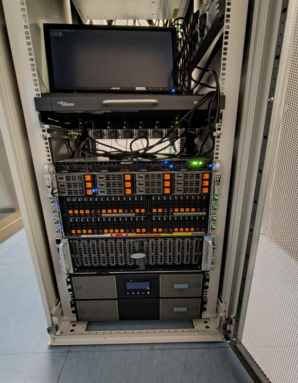
In addition, for development and testing, CNR-IAC acquired a Dell Server R940 – NVME with four Xeon Gold 6252N processors each with 24 cores, and 1Tb RAM.
Software:
The available open software installed and characterized includes several radiative transfer models, among which:
- The accurate KLIMA model developed maintained at CNR-IFAC (see Del Bianco, S.; Carli, B.; Gai, M.; Laurenza, L.M.; Cortesi, U. XCO2 retrieved from IASI using KLIMA algorithm. Ann. Geophys., 56. https://doi.org/10.4401/ag-6331, 2014)
- The fast Radiative Transfer model for TOVs (RTTOV, https://nwp-saf.eumetsat.int/site/software/rttov/) with its hyper-fast variant using the Principal Components analysis (PC-RTTOV).
- The σ-IASI/F2N code developed at the Universities of Basilicata and Bologna (https://zenodo.org/records/7019991)
- The Rapid Radiative Transfer Model (RRTM) http://rtweb.aer.com/rrtm_frame.html developed by the AER company in the US
- The ECMWF radiation scheme eCrad (https://confluence.ecmwf.int/display/ECRAD)
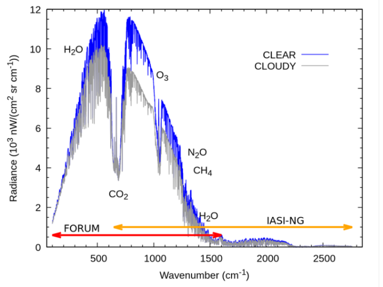
- The CLAIM (Clouds and Atmosphere Inversion Module), the retrieval code of the Far-Infra-Red Outgoing Radiation Understanding and Monitoring – End-to-End simulator (FORUM E2E) project (https://amt.copernicus.org/articles/15/573/2022/) , based on Line-by-line Radiative Transfer Module (LBLRTM) (https://github.com/AER-RC/LBLRTM) and DIScrete Ordinate Radiative Transfer (DISORT) (http://www.rtatmocn.com/disort). The figure below shows examples of simulated spectrally resolved radiances upwelling at the top of the atmosphere (TOA), for clear and cloudy sky atmospheres.
In addition, within the infrastructure project, we also developed tools for spectral fluxes computation
(angular integration of spectral radiance) and tools for instrument spectral response function convolutions.
Comparison of Fast Radiative Transfer Models
The radiative transfer tools installed at the CNR-INO computing facility were characterized from both the point of view of accuracy and speed. The accuracy of the models was assessed by comparison of the spectral radiances or the band-specific fluxes to analogous calculations carried out with the slow and accurate KLIMA model.
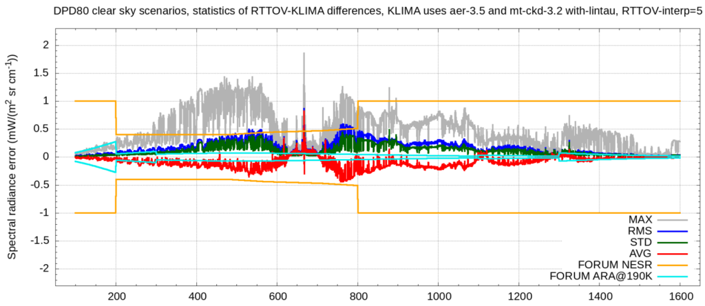
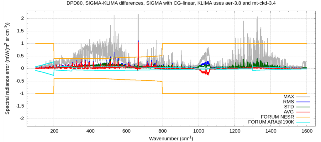
Figures above show example results of the intercomparisons between RTTOV and KLIMA and between σ-IASI/F2N and KLIMA, respectively.
The two codes were also analyzed from the algorithmic point of view. The characteristics of the two codes are summarized in the following Table.
Characteristic | RTTOV | σ-IASI/F2N |
Development | Large development team and community. Already used in meteorological models | Small community and development team, almost all Italian |
Algorithm (clear sky) | Fully parametric | Series expansion |
Algorithm (cloudy sky) | Fully parametric | Chu+Tang physical models |
Product | Instrumental radiance | Hi-res radiance and instrument radiance after convolution with the ISRF |
Number of variable gases | Depending on the predictors. Max 7 for most instruments. | Max 12 gases. |
Accuracy | For FORUM: about 100% of ARA | For FORUM: about 40% of ARA. |
Insertion in a climatological or meteorological model | Easy. | Only as an external executable. |
RT of single spectral channels | YES | NO |
Numerical Optimization | Already performed | Ample margin |
Further Optimization | Using the PC-RTTOV version | Ample margin |
The most important characteristic is the possibility of performing the radiative transfer of single channels, which is essential in assimilation. The RTTOV code can do it, because the convolution with the ISRF is already factored in the pre-recorded coefficients table, while the σ-IASI/F2N needs to perform a convolution, so that a whole neighborhood of each frequency is needed.
The RTTOV can be further optimized by using the PC-RTTOV version due to Matricardi (https://rmets.onlinelibrary.wiley.com/doi/10.1002/qj.680). PC-RTTOV is able to reconstruct a full IASI spectrum (8461 spectral channels) using only a subset of channels (called scores) and a linear operation. In the figure below we report the error pertaining to the whole spectral reconstruction using 50, 200 and 300 scores, compared with the IASI random noise.
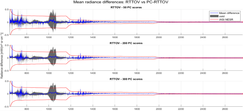
The computational time of PC-RTTOV using 200 scores is about 1/10 of that of the full RTTOV radiative transfer.
Outgoing long-wave fluxes
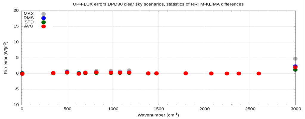
The spectral radiances produced by KLIMA and σ-IASI/F2N were also angularly integrated (with a newly developed tool) to get the down-welling and the up-welling energy fluxes in specific spectral bands. The obtained fluxes were then compared to those generated by the RRTM and the eCrad codes.
Here is an example of the intercomparison between KLIMA and RRTM derived fluxes. While faster than KLIMA by several orders of magnitude, RRTM provides total long-wave fluxes with accuracy of the order of 1-2 W/m2.
Speed intercomparisons
The following table summarizes the computing times required by the radiative transfer codes computing spectrally resolved radiances (KLIMA, σ-IASI/F2N and RTTOV).
RTM code | Elapsed time | CPU time |
KLIMA | ~ 1200 hours | 43.2 * 105 s |
SIGMA-IASI | 104 s | 45 s |
RTTOV | 8.6 s | 7.6 s |
The RRTM and eCrad codes compute only the band-integrated and total fluxes and are usually embedded in global models that call them billions of times within a single model run. Thus, while more inaccurate, these codes are, by far, faster than both RTTOV and σ-IASI/F2N.
Applications and know-how
Using the characterized radiative transfer models described earlier, we are able to build the end-to-end (E2E) chain (from data acquisition to Level 2 geophysical products) for the simulation of atmospheric passive remote sensing missions. The E2E simulation allows to characterize the product quality as a function of the measurement characteristics, thus it is extremely useful to set up the requirements in the initial phases of a new mission.
Conversely, given the accuracy, the precision and the geometrical specifications of a future or a already running mission, we can assess the information contained in the measurements and the possibility to derive new geophysical products.
Artificial Intelligence methods
Due to the large volume of data expected from next-generation sensors, new machine learning (ML) approaches have been proposed. Although these approaches must rely on physical models during the training phase, the algorithms themselves, typically based on architectures such as neural networks, learn a functional relationship directly from previously generated results of the same or similar problems.
In principle, ML methods can replace any full-physics procedure. However, in the field of remote sensing, research has mainly focused on three application areas:
- Scene classification, such as distinguishing between clear and cloudy conditions, or estimating indices related to scene homogeneity and cloudiness.
- The forward model, i.e. predicting a spectrum from a given atmospheric state (radiative transfer, RT).
- The inverse problem, i.e. retrieving the atmospheric state from measurements (retrieval).
Scene classification is important because the presence of clouds requires the use of radiative transfer models that account for multiple scattering. Modern instruments are often complemented by ancillary sensors for analyzing the field of view, and some instruments are specifically designed for cloud detection and characterization.
A major challenge for ML approaches applied to the RT problem is the curse of dimensionality. An atmospheric state may be described by hundreds of parameters, while the corresponding spectral radiance can consist of thousands of channels. In full-physics models, correlations between spectral channels are inherently represented. In contrast, ML models must learn these correlations from the training data set, which is a demanding task.
For the retrieval problem, the main difficulty lies in the ill-posed nature of the inversion. Full-physics retrieval methods address this issue through regularization techniques, such as reducing dimensionality using Principal Component Analysis (PCA), or constraining solutions towards a climatological prior. ML approaches must incorporate similar strategies, either by learning appropriate regularization from the training dataset or by projecting both atmospheric states and radiances into lower-dimensional spaces (latent spaces) and learning relationships between these representations (e.g. latent twin approaches).
Although ML methods offer very fast inference once trained, their retrieval accuracy still generally falls short of that achieved by full-physics approaches. Ongoing research aims to improve their precision, potentially making them a viable alternative to more computationally expensive methods.
WP-1500.5 – Improving the representation of radiative fluxes in global climate models
Scientific and infrastructural objectives:
Radiative fluxes are a fundamental element in understanding the Earth’s climate system, as they govern the planet’s energy balance and the direct response to greenhouse gas forcing, the main driver of current climate change. In this delicate balance between absorbed and re-emitted energy, clouds play a pivotal role: their presence alters the net radiative balance by approximately 20 W/m², a significant figure when compared to the current imbalance of around 0.7 W/m² that is warming the planet. Precisely for this reason, in order for climate models to provide reliable future projections, it is essential that they accurately calculate these energy fluxes. However, the representation of clouds within models remains one of the major sources of scientific uncertainty, due to the spatial scales and the complexity of the microphysical processes involved.
It is within this context that the activities of this module take place, the primary objective of which is the development of climate models and the analysis of systematic biases affecting the simulation of radiative fluxes and their variability, with particular attention to the representation of clouds. In parallel, the module deals with the simulation of historical climate and future scenarios, producing atmospheric fields (e.g. radiative fluxes, temperature/humidity profiles, cloud distribution) for comparison with observations.
In its first two years of operation, the module’s main focus was the development of the climate version of the GLOBO model, an atmospheric model developed at CNR-ISAC for weather forecasting and recently adapted for the study of the climate system on seasonal/decadal scales (https://git.isac.cnr.it/esm/globone). Applications dedicated to the interface between the model and observations, on the other hand, centre on the EC-Earth climate model, developed within a European consortium of which CNR-ISAC is a core partner.
Context within the EMN component
The module is part of the EMN – Earth and Mars Research Network component and falls within the scope of meteorological and climate modelling activities. Interaction with the other components of the infrastructure aims to harness the potential of future Earth observations (e.g. FORUM or LETO) in analysing the climate system’s radiative response to anthropogenic forcing. The module provides a framework for exploring, on the one hand, the opportunities offered by specific observations for understanding model shortcomings and, on the other, through projections across various future scenarios, the impact of future observations on the study of climate feedbacks.
Functional Units
1. HPC Cluster
The module has at its disposal a parallel computing cluster for climate modelling, with a dedicated GPU server. The system consists of 16 computing nodes (64 CPUs each), a storage system (200 TB) and a GPU node (3 A30 GPUs). The cluster is available to the infrastructure for model development and testing, for the production and storage of climate simulations, and for activities related to the interface with observations.
2. Simulation of historical climate and future scenarios
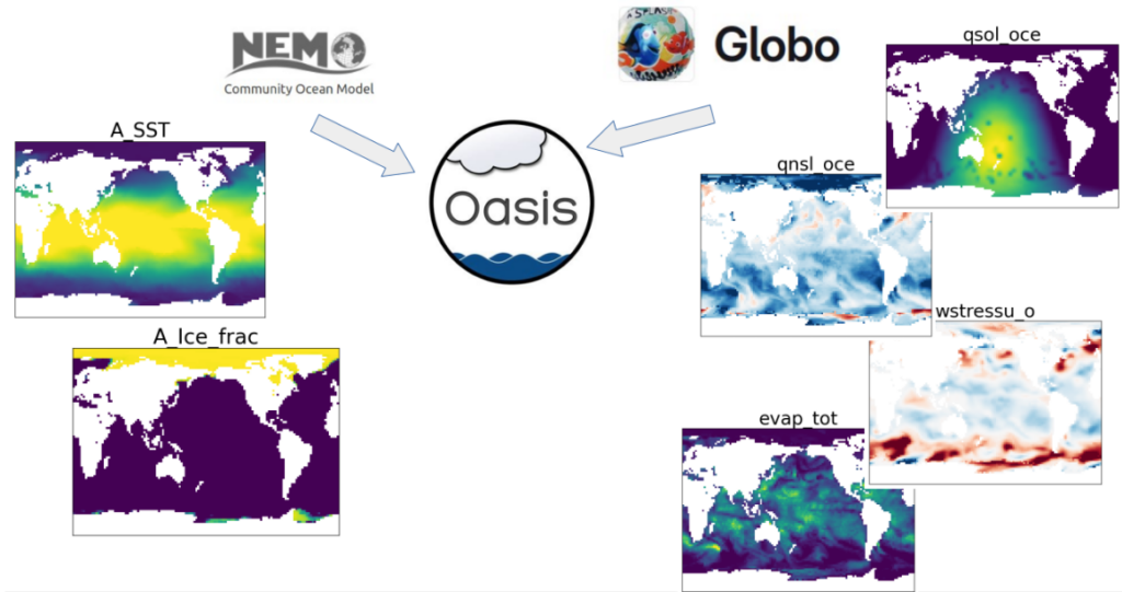
The module utilises two main modelling tools. GLOBO is a general atmospheric circulation model developed over 30 years at CNR-ISAC, now updated in its radiative parameterisation and prepared for coupling with the NEMO ocean model – in collaboration with CNR-ISMAR – for seasonal and decadal-scale simulations and climate scenarios. The coupled model is currently under development, but a preliminary version is available via the institute’s repository: https://git.isac.cnr.it/esm/globone.
EC-Earth is a coupled climate model, consisting of the openIFS model for its atmospheric component (developed at the ECMWF) and the NEMO ocean model. EC-Earth participated in the last two phases of the CMIP (Coupled Model Intercomparison Project) initiative and will participate in the next phase (CMIP7) with the EC-Earth4 model.
Contribution of the module to the EMN infrastructure
The module forms part of the EMN component within the field of meteorological and climate modelling, acting as a bridge between numerical climate simulation and future Earth observation missions, such as FORUM or LETO. Interaction with other elements of the infrastructure is aimed at leveraging new observational capabilities in the analysis of the system’s radiative response to anthropogenic forcing. In this regard, the module provides an operational framework capable of operating on two complementary fronts: on the one hand, it allows us to explore how specific observations can help diagnose and address current shortcomings in climate models; on the other, through the simulation of different emission scenarios, it enables us to assess the concrete impact that such observations will have on our understanding of climate feedbacks.